
I. The Problem with Naïve Expected-Value Sizing
Consider a repeatable, positive-edge bet. The naïve instinct is to size it by maximizing expected wealth after a single round:
E[W1] = W0 · [1 + f · (pb − q)]
Where f is the fraction of bankroll wagered, p is win probability, q = 1−p, and b is the net odds. This expression is linear in f, and its slope is positive whenever the bet has positive edge (pb > q). A linear function with positive slope is maximized at the boundary, so naïve maximization says: bet everything, every round. This is in fact wrong, and the reason it is wrong is structural. At f=1, a single loss sets wealth to zero, and a portfolio cannot recover at zero. The criterion is scoring one round in isolation when the actual object of interest is what happened under repetition.
II. Why the Correct Criterion is E[log(Wealth)]
This is the part most retail explanations get wrong: they present log-utility as a preference assumption (as if a Kelly bettor simply prefers log-shaped utility). It is not a preference assumption, but rather a consequence of how wealth compounds under repetition, provable from the Strong Law of Large Numbers alone.
Wealth after T rounds of a repeated bet compounds multiplicatively:
WT = W0 · ∏i=1T (1 + f · Ri)
Take logs of both sides:
ln(WT) = ln(W0) + Σi=1T ln(1 + f · Ri)
The summands ln(1 + f · Ri) are i.i.d. across rounds (same bet repeated). By the Strong Law of Large Numbers:
(1/T) · ln(WT/W0) → E[ln(1 + f · R)] almost surely, as T → ∞
Define g(f) := E[ln(1 + f · R)], the asymptotic per-round compound growth rate as a function of bet size. Whatever f maximizes g(f) is, with probability 1, the sizing rule that produces the highest long-run wealth and gets there fastest. This is Kelly’s original 1956 result. It was placed on rigorous footing as a growth-optimality theorem by Breiman (1961) and it holds regardless of the bettor’s actual risk preferences because it is a statement about the almost-sure limiting behavior of a multiplicative stochastic process.
Concavity (so the optimum is real and unique): for fixed R, h(f) = ln(1+f · R) is a concave function composed with an affine argument, hence concave in f. Expectation preserves concavity (Jensen), so g(f) = E[h(f)] is concave in f. This guarantees a unique global maximum reachable by standard first-order conditions.
III. Deriving f* for a Simple Binary Bet
Win w.p. p → wealth ×(1+f · b). Lose w.p. q → wealth ×(1−f).
g(f) = p · ln(1+fb) + q · ln(1−f)
First-order condition:
- g′(f) = pb/(1+fb) − q/(1−f) = 0
- pb(1−f) = q(1+fb)
- pb − q = fb(p+q) = fb [since p+q=1]
- f* = (pb − q)/b = p − q/b
This is the classical closed-form Kelly fraction, specifically because the payoff has exactly two outcomes.
IV. Application: Kalshi Binary Markets
A Kalshi YES contract settling at $1/$0, priced at c (implied probability), gives net odds b = (1−c)/c. Substituting into f* = (pb−q)/b:
f* = [p · (1−c)/c − (1−p)] / [(1−c)/c] = (p − c)/(1 − c)
This is not a separate formula; it is the identical growth-optimal derivative, evaluated at the odds structure a Kalshi contract happens to have.
V. Why Credit Spreads Break the Closed-Form Case
A vertical credit spread’s payoff is not two clean outcomes. Take a concrete short put spread: short strike Ks, long strike Kl (Kl < Ks), credit received C, width W = Ks − Kl, max risk = W − C. At expiration, P&L as a function of terminal price S:
- S ≥ Ks: both legs expire worthless → P&L = +C (capped)
- Kl < S < Ks: short leg ITM, long leg still OTM → P&L = C − (Ks − S), a full continuum
- S ≤ Kl: both legs ITM → P&L = C − W (capped)
This is piecewise-linear in S, with kinks at both strikes, which is not binary. Therefore, the growth function generalizes to:
g(f) = ES[ln(1 + f · R(S))], where R(S) = P&L(S) / (W − C) (return on max-risk capital)
To evaluate this expectation, we need a distributional model for terminal price S. The natural choice consistent with how the rest of the book already prices options is the lognormal (GBM) assumption Black-Scholes makes:
ST = S0 · exp[(μ − σ2/2)T + σ√T · Z], where Z ~ N(0,1)
g(f) = ∫ ln(1 + f · R(ST(z))) · φ(z) dz, where φ is the standard normal density
Because R(S) is piecewise-linear (not a step function), this integral has no closed form. f* must be found numerically: evaluate g(f) over a grid and take the argmax. Concavity from Section II still guarantees this argmax is unique and well-defined.
VI. Critical Insight: Kelly Needs a Subjective Edge, Not the Market’s Own Pricing
This is the point that separates a real quant treatment from a mechanical one. If you simulate ST using σ = implied volatility and μ = risk-free rate r (i.e., the actual Black-Scholes risk-neutral measure the option was priced under), the Fundamental Theorem of Asset Pricing guarantees E[P&L] = 0. Under that measure, that is the definition of a fair, arbitrage-free price. Kelly sizing under a genuinely zero-edge input correctly returns f* ≈ 0: size nothing. A Kelly calculation that spits out a large position size while secretly assuming the market’s own risk-neutral pricing is internally contradicting, as it is borrowing an edge from nowhere.
A non-zero f* requires a genuine, defensible subjective view that departs from the market’s own pricing. For an options-selling book such as AJAX’s, the standard, empirically grounded departure is the variance risk premium: implied volatility has run structurally above subsequently-realized volatility across four decades of data (CBOE PUT-Index, Bakshi & Kapadia 2003, Carr & Wu 2009, AQR’s isolated-VRP-factor study). Substituting σsubjective (a realistic, empirically calibrated realized-vol estimate) < σimplied, while holding drift at μ = r (expressing no directional view, particularly isolating the vol-selling edge in isolation), is what turns this into an actual sizing tool grounded in a real and testable edge.
VII. Worked Example: GS $990/$1000 Put Spread (Live Data, 2026-07-20)
Current chain (Aug 21 expiry): 1000P mid ≈ $19.875, 990P mid ≈ $16.975 → C = $290, W = $1,000, max risk = $710. Spot S0 = $1,055.03, T = 32/365, r = 3.7%. Average implied vol on these strikes ≈ 35.0%.
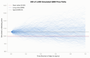
With a single vol applied consistently across both legs, mean(R) ≈ -0.0038 and f* ≈ 0.000, which is effectively zero, exactly as Section VI predicts. Simulating at σ = implied, μ = r reproduces the market’s own risk-neutral measure, under which the Fundamental Theorem of Asset Pricing guarantees E[P&L] = 0; a non-zero edge requires the subjective departure introduced next.
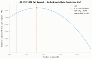
Subjective case: GS’s pre-earnings (i.e., “normal regime,” excluding the July 14 event) 60-day realized vol was 31.3% vs. 35% implied. That ~3.7% vol-point gap is the actual defensible edge (the VRP, measured directly on this name). Re-running with σ = 31.3%, μ = r:
- f* ≈ 0.08, mean(R) ≈ +0.0324
That is: full Kelly says risk ~8% of bankroll as max-risk-capital on this single spread. On a $1 million book (income sleeve), that is roughly $80,000. Clearly, this is too aggressive for a single position (full Kelly always is); see Section VIII.
| Sizing Rule | % of Book | Max Risk Capital | Approx. Contracts ($710 max risk each) |
|---|---|---|---|
| Full Kelly | ~8% | $80,000 | ~113 |
| Half-Kelly | ~4% | $40,000 | ~56 |
| Quarter-Kelly | ~2% | $20,000 | ~28 |
Kelly is applied here against the capital dedicated to the income sleeve, not total NAV. This is a deliberate simplification of the full multi-asset Kelly problem (Section IX): true joint optimization would size every position in the portfolio simultaneously, accounting for cross-strategy correlation, which is both statistically intractable to estimate reliably and strategically undesirable. Capital should stay segmented by strategy type rather than be freely reallocated by an optimizer. This framing implicitly assumes the income sleeve’s outcomes are close to uncorrelated with the core equity book, which is a reasonable approximation for defined-risk short-dated options spreads against a longer-horizon equity book, but not an exact one. Note also that the sizing of the carve-out itself (what % of NAV goes to the income sleeve) is a separate decision, made outside the Kelly framework. Kelly only answers how to size within an already-chosen budget, not what that budget should be.
VIII. Why Fractional Kelly and Not Full Kelly
Full Kelly is provably growth-optimal if the inputs (p, σ, edge) are exactly correct. In practice, they are estimates, and g(f) is sharply asymmetric around its peak: overestimating f* costs growth rate much faster than underestimating it by the same amount. In the continuous-time (diffusion) approximation, the growth rate as a function of leverage is exactly quadratic:
g(f) = A · f − B · f2, giving f* = A/(2B) and g(f*) = B · f*2.
Evaluating at a fraction k of full Kelly:
g(k · f*)/g(f*) = k(2−k)
At k = 0.5 (half-Kelly): retains 0.5×1.5 = 75% of the growth rate, for a large cut in variance and in the consequences of a misestimated edge. This is the exact justification for the half/quarter-Kelly output.
IX. Limitations
- This derivation sizes one isolated repeated bet. The actual book runs multiple concurrent spreads across different underlyings simultaneously. A true portfolio-level Kelly requires a covariance-adjusted multi-asset generalization (analogous in spirit to Markowitz mean-variance optimization), not independent single-bet Kelly calculations stacked side by side.
- Ignores transaction costs, bid-ask execution slippage, and early-assignment/American-exercise risk on short leg.
- The subjective σ input (realized vol) is itself an estimate with its own uncertainty. Essentially, garbage in, garbage out still applies; Section VIII’s fractional-Kelly discipline is the mitigation, not a fix for a badly wrong edge estimate.
References
- Kelly, J. L. (1956). “A New Interpretation of Information Rate.” Bell System Technical Journal, 35(4), 917–926.
- Breiman, L. (1961). “Optimal Gambling Systems for Favorable Games.” Proceedings of the Fourth Berkeley Symposium on Mathematical Statistics and Probability, Vol. 1, 65–78.
- Bakshi, G., & Kapadia, N. (2003). “Delta-Hedged Gains and the Negative Market Volatility Risk Premium.” The Review of Financial Studies, 16(2), 527–566.
- Carr, P., & Wu, L. (2009). “Variance Risk Premiums.” The Review of Financial Studies, 22(3), 1311–1341.
- AQR Capital Management. (2018). “Understanding the Volatility Risk Premium.” AQR White Paper.
- Bondarenko, O. (2019). “Historical Performance of Put-Writing Strategies.” CBOE Research.
